Visualization & Analysis - Crowd Sound Project

This notebook loads the extracted features and produces:

Feature inspection (ranked sounds per feature)
Boxplots: F0 and spectral centroid by group (A vs J)
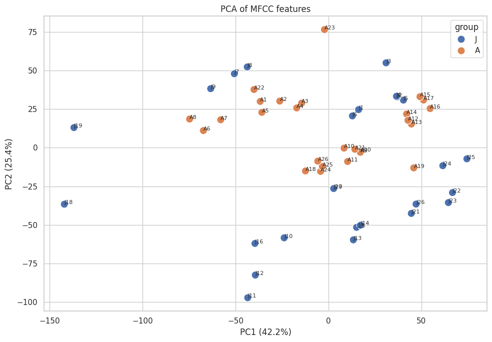
PCA of MFCC features
K-Means clustering (unsupervised, k=2)

Imports¶

import os
import json
import numpy as np
import pandas as pd
import seaborn as sns
import matplotlib.pyplot as plt
from sklearn.cluster import KMeans
from sklearn.decomposition import PCA

Load Data¶

outputs_folder = "../outputs"
figures_folder = "../figures"
os.makedirs(figures_folder, exist_ok=True)

data = []
for sound_folder in os.listdir(outputs_folder):
    json_path = os.path.join(outputs_folder, sound_folder, "results.json")
    if os.path.exists(json_path):
        with open(json_path, "r") as f:
            result = json.load(f)
            result["file"] = sound_folder
            result["group"] = sound_folder[0]
            data.append(result)

df = pd.DataFrame(data)
print(f"Loaded {len(df)} sounds")
df.head()

Loaded 52 sounds

Feature Inspection¶

Sounds ranked by acoustic feature values — identifies the most and least extreme sounds in the dataset.

df_sorted_f0 = df.sort_values(by="f0_mean", ascending=False)
df_sorted_centroid = df.sort_values(by="spectral_centroid_mean", ascending=False)
df_sorted_bandwidth = df.sort_values(by="spectral_bandwidth_mean", ascending=False)
df_sorted_rolloff = df.sort_values(by="spectral_rolloff_mean", ascending=False)

print("Highest F0:"); print(df_sorted_f0[["file", "f0_mean"]].head(3).to_string(index=False))
print("\nHighest spectral centroid:"); print(df_sorted_centroid[["file", "spectral_centroid_mean"]].head(3).to_string(index=False))
print("\nLowest F0:"); print(df_sorted_f0[["file", "f0_mean"]].tail(3).to_string(index=False))
print("\nLowest spectral centroid:"); print(df_sorted_centroid[["file", "spectral_centroid_mean"]].tail(3).to_string(index=False))

# Save inspection JSON
inspection_results = {
    "highest_f0": df_sorted_f0[["file", "f0_mean"]].head(5).to_dict(orient="records"),
    "lowest_f0": df_sorted_f0[["file", "f0_mean"]].tail(5).to_dict(orient="records"),
    "highest_spectral_centroid": df_sorted_centroid[["file", "spectral_centroid_mean"]].head(5).to_dict(orient="records"),
    "lowest_spectral_centroid": df_sorted_centroid[["file", "spectral_centroid_mean"]].tail(5).to_dict(orient="records"),
    "highest_spectral_bandwidth": df_sorted_bandwidth[["file", "spectral_bandwidth_mean"]].head(5).to_dict(orient="records"),
    "lowest_spectral_bandwidth": df_sorted_bandwidth[["file", "spectral_bandwidth_mean"]].tail(5).to_dict(orient="records"),
    "highest_spectral_rolloff": df_sorted_rolloff[["file", "spectral_rolloff_mean"]].head(5).to_dict(orient="records"),
    "lowest_spectral_rolloff": df_sorted_rolloff[["file", "spectral_rolloff_mean"]].tail(5).to_dict(orient="records")
}
with open("../outputs/feature_inspection.json", "w") as f:
    json.dump(inspection_results, f, indent=4)
print("\nFeature inspection JSON saved")

Highest F0:
file    f0_mean
 J21 443.329615
 J26 440.971992
 J24 440.303943

Highest spectral centroid:
file  spectral_centroid_mean
 J23             3082.449785
 J22             3071.324966
 J25             3059.090960

Lowest F0:
file    f0_mean
 A11 133.956327
 A23 120.365753
 A22 119.143413

Lowest spectral centroid:
file  spectral_centroid_mean
  A8             1462.277867
 A22             1382.109020
 A23             1305.430443

Feature inspection JSON saved

Boxplots by Group¶

Comparison of F0 and spectral centroid distributions between Group A and Group J.

sns.set(style="whitegrid")

fig, axes = plt.subplots(1, 2, figsize=(14, 6))

sns.boxplot(data=df, x="group", y="f0_mean", ax=axes[0])
axes[0].set_title("F0 mean by group")
axes[0].set_xlabel("Group")
axes[0].set_ylabel("F0 mean (Hz)")

sns.boxplot(data=df, x="group", y="spectral_centroid_mean", ax=axes[1])
axes[1].set_title("Spectral centroid by group")
axes[1].set_xlabel("Group")
axes[1].set_ylabel("Spectral centroid")

plt.tight_layout()
plt.savefig("../figures/boxplots_by_group.png", dpi=150)
plt.show()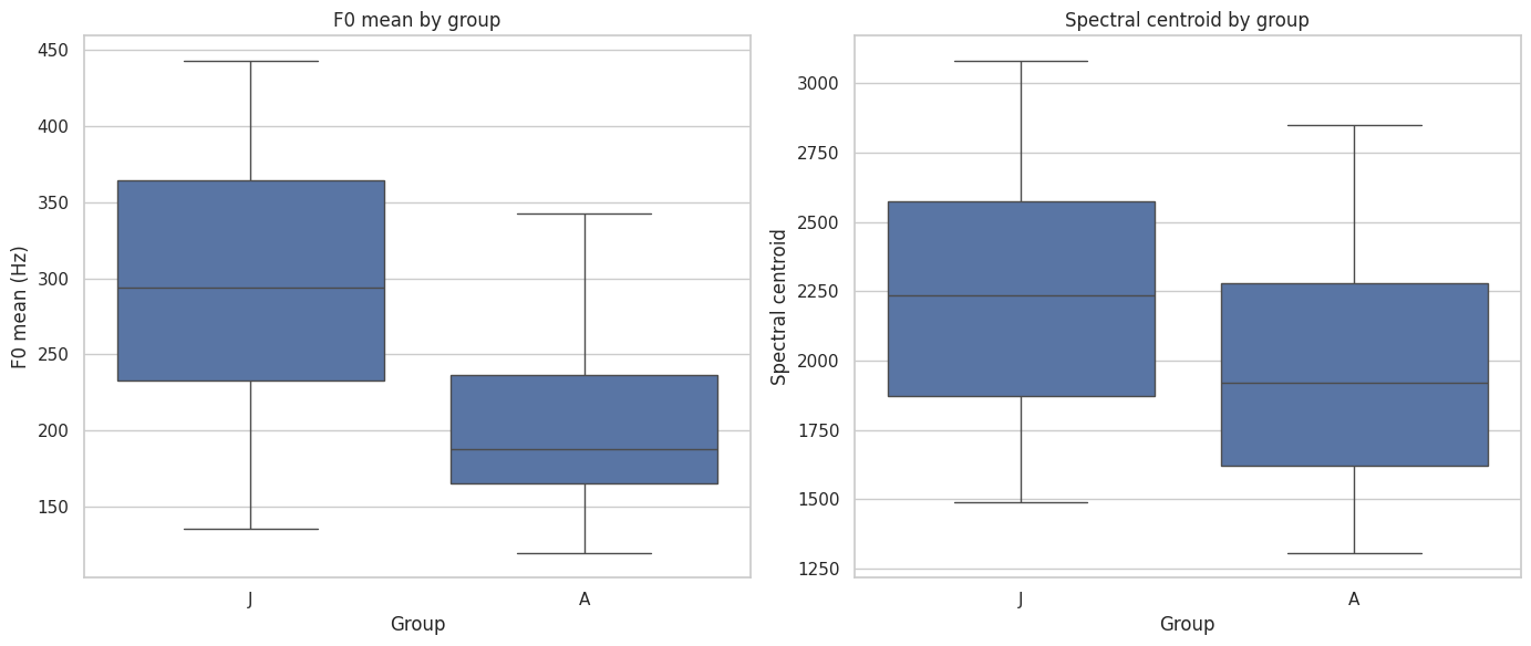

PCA on MFCC Features¶

Principal Component Analysis reduces the 13 MFCC coefficients to 2 dimensions for visualization. Each point is one sound, colored by group.

mfcc_data = [item["mfcc_mean"] for item in data]
labels = [item["group"] for item in data]
files = [item["file"] for item in data]

X = np.array(mfcc_data)
pca = PCA(n_components=2)
X_pca = pca.fit_transform(X)

df_pca = pd.DataFrame({
    "pc1": X_pca[:, 0],
    "pc2": X_pca[:, 1],
    "group": labels,
    "file": files
})

print(f"Variance explained: PC1={pca.explained_variance_ratio_[0]:.1%}, PC2={pca.explained_variance_ratio_[1]:.1%}")

plt.figure(figsize=(10, 7))
sns.scatterplot(data=df_pca, x="pc1", y="pc2", hue="group", s=120)
for i, row in df_pca.iterrows():
    plt.text(row["pc1"], row["pc2"], row["file"], fontsize=8)
plt.title("PCA of MFCC features")
plt.xlabel(f"PC1 ({pca.explained_variance_ratio_[0]:.1%})")
plt.ylabel(f"PC2 ({pca.explained_variance_ratio_[1]:.1%})")
plt.tight_layout()
plt.savefig("../figures/pca_mfcc_individual.png", dpi=150)
plt.show()

Variance explained: PC1=42.2%, PC2=25.4%

K-Means Clustering¶

Unsupervised clustering (k=2) applied to MFCC features — tests whether the algorithm can recover the A/J groups without using the labels.

kmeans = KMeans(n_clusters=2, random_state=42, n_init=10)
clusters = kmeans.fit_predict(X)
df_pca["cluster"] = clusters.astype(str)

plt.figure(figsize=(10, 7))
sns.scatterplot(data=df_pca, x="pc1", y="pc2", hue="cluster", palette="Set1", s=120)
for i, row in df_pca.iterrows():
    plt.text(row["pc1"], row["pc2"], row["file"], fontsize=8)
plt.title("K-Means clustering on MFCC (k=2, unsupervised)")
plt.xlabel(f"PC1 ({pca.explained_variance_ratio_[0]:.1%})")
plt.ylabel(f"PC2 ({pca.explained_variance_ratio_[1]:.1%})")
plt.tight_layout()
plt.savefig("../figures/kmeans_mfcc.png", dpi=150)
plt.show()

print("Done — all figures saved")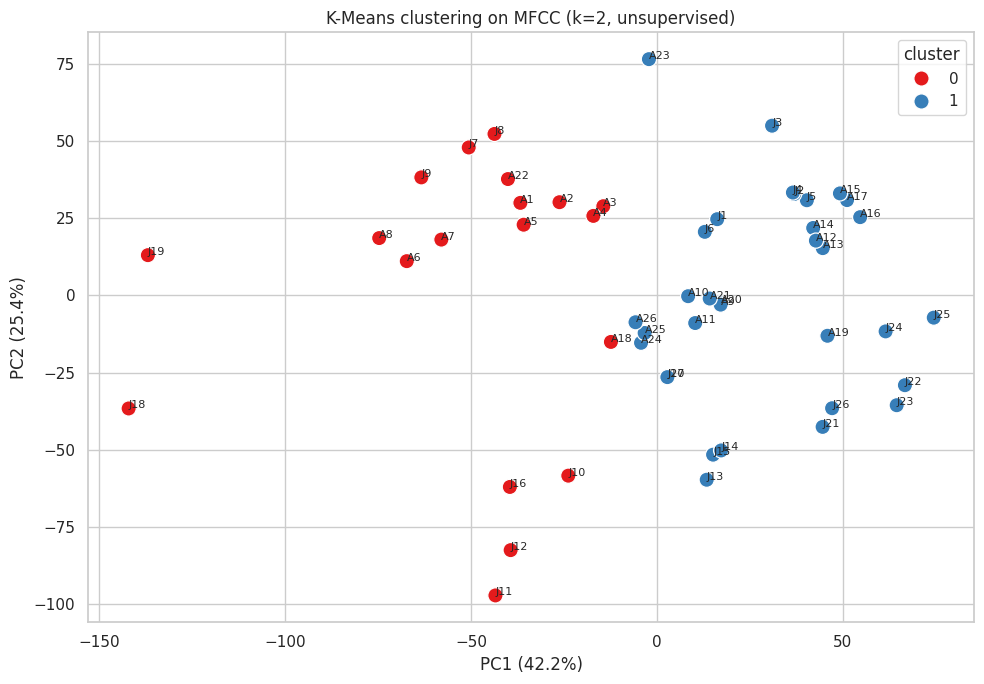

Done — all figures saved